m(n) map

m(n) map
Based on	\(f^x(x)\)
Growth rate	\(f_{\varepsilon_0}(n)\)

m(n) map is a googological function that operates on functions. It was defined by Japanese googologist Fish in 2003 and used to define Fish number 5. Its system achieves a growth rate of \(f_{\varepsilon_0}(n)\), similar to Hydra function and tetrational array of BEAF. The name of the map was taken from a word mapping.

Definition and growth rate

Each \(m(n)\) is a function with an identical domain and codomain. \(m(1)\) has domain and codomain \(\mathbb{N}\), and each \(m(n + 1)\) is \((D \mapsto D) \mapsto (D \mapsto D)\), where \(D\) is the (co)domain of \(m(n)\). So \(m(1) : \mathbb{N} \mapsto \mathbb{N}\), \(m(2) : (\mathbb{N} \mapsto \mathbb{N}) \mapsto (\mathbb{N} \mapsto \mathbb{N})\), \(m(3) : ((\mathbb{N} \mapsto \mathbb{N}) \mapsto (\mathbb{N} \mapsto \mathbb{N})) \mapsto ((\mathbb{N} \mapsto \mathbb{N}) \mapsto (\mathbb{N} \mapsto \mathbb{N}))\), and so forth.

\begin{eqnarray*} m(1)(x) & = & x^x \\ m(2)f(x) & = & f^x(x) \end{eqnarray*}

where \(m(2)\) matches \(s(1)\) of s(n) map; \(m(2)=s(1)\).

\(m(3)\) map is a function which maps "function which maps functions to function" to "function which maps functions to function", defined and calculated as (parenthesis is written verbosely here to indicate the order of calculation)

\begin{eqnarray*} ((m(3)m(2))f)(x) & = & (m(2)^xf)(x) \\ & = & (s(1)^xf)(x) \\ & = & (s(2)f)(x) \end{eqnarray*} Therefore, \(m(3) m(2) = s(2)\) in \(s(x)\) map, and \(m(3)^2 m(2)\) is calculated as \(s(3)\) as follows. \begin{eqnarray*} ((m(3)^2m(2))f)(x) & = & ((m(3)(m(3)m(2)))f)(x) \\ & = & ((m(3)m(2))^xf)(x) \\ & = & (s(2)^xf)(x) \\ & = & (s(3)f)(x) \end{eqnarray*}

Calculation goes on similarly, with FGH approximation,

\begin{eqnarray*} m(3)^3 m(2) m(1)(x) & = & s(4)f(x) \approx f_{\omega^3}(x) \\ m(3)^4 m(2) m(1)(x) & = & s(5)f(x) \approx f_{\omega^4}(x) \\ m(3)^n m(2) m(1)(x) & = & s(n+1)f(x) \approx f_{\omega^n}(x) \\ m(3)^x m(2) m(1)(x) & = & s(x)f(x) \approx f_{\omega^\omega}(x) \\ \end{eqnarray*}

where \(f(x) = m(1)(x) = x^x\). In general

• \(M_0\) = set of positive integers
• \(M_{n+1}\) = set of functions which map \(M_n\) to \(M_n\)

\(m(n)\) map \((n \ge 1)\) belongs to \(M_n\) and is defined as follows.

For \(f_n \in M(n)\), \(m(n+1)(f_n) = g_n\) is defined as follows.

For \(f_{n-1} \in M(n-1)\), \(g_n(f_{n-1}) = g_{n-1}\) is defined as follows.

For \(f_{n-2} \in M(n-2)\), \(g_{n-1}(f_{n-2}) = g_{n-2}\) is defined as follows.

……

For \(f_0 \in M(0)\), \(g_1(f_0) = g_0\) is defined as follows.

\(g_0 = (..((f_n^{f_0}f_{n-1})f_{n-2})...f_1)f_0\)

Therefore, by denoting \(f_1\) as \(f\) and \(f_0\) as \(x\), \begin{eqnarray*} m(1)(x) & = & {x}^{x} \\ (m(2)f)(x) & = & ({f}^{x})(x) \\ ((..((m(n+1)f_n)f_{n-1})...f_2)f)(x) & = & ((..({f_n}^{x}{f_{n-1}})...f_2)f)(x) \end{eqnarray*}

And it works out like this.

\begin{eqnarray*} m(4) m(3) m(2) m(1)(x) & = & m(3)^x m(2) m(1)(x) \approx f_{\omega^\omega}(x) \\ m(3) [m(4) m(3)] m(2) m(1)(x) & = & [m(3)^{x} m(2)]^x m(1)(x) \approx f_{\omega^{\omega+1}}(x) \\ m(3)^2 [m(4) m(3)] m(2) m(1)(x) & \approx & f_{\omega^{\omega+2}}(x) \\ m(3)^a [m(4) m(3)] m(2) m(1)(x) & \approx & f_{\omega^{\omega+a}}(x) \\ [ m(4) m(3) ] ^2 m(2) m(1)(x) & = & [ m(3)^x ] [ m(3)^x m(2)] m(1)(x) \approx f_{\omega^{\omega \times 2} } (x) \\ [ m(4) m(3) ] ^3 m(2) m(1)(x) & \approx & f_{\omega^{\omega \times 3} } (x) \\ [ m(4) m(3) ] ^a m(2) m(1)(x) & \approx & f_{\omega^{\omega \times a} } (x) \\ [ m(4)^2 m(3) ] m(2) m(1)(x) & \approx & f_{\omega^{\omega^2} } (x) \\ m(3) \bigl[ m(4)^2 m(3) ] m(2) m(1)(x) & \approx & f_{\omega^{\omega^2+1} } (x) \\ [ m(4) m(3) ] [ m(4)^2 m(3) ] m(2) m(1)(x) & \approx & f_{\omega^{\omega^2+\omega} } (x) \\ [ m(4) m(3) ] ^2 [ m(4)^2 m(3) ] m(2) m(1)(x) & \approx & f_{\omega^{\omega^2+\omega \times 2} } (x) \\ [ m(4) m(3) ] ^3 [ m(4)^2 m(3) ] m(2) m(1)(x) & \approx & f_{\omega^{\omega^2+\omega \times 3} } (x) \\ [ m(4)^2 m(3) ] ^2 m(2) m(1)(x) & \approx & f_{\omega^{\omega^2 \times 2} } (x) \\ [ m(4)^2 m(3) ] ^3 m(2) m(1)(x) & \approx & f_{\omega^{\omega^2 \times 3} } (x) \\ m(4)^3 m(3) m(2) m(1)(x) & \approx & f_{\omega^{\omega^3} } (x) \\ m(4)^4 m(3) m(2) m(1)(x) & \approx & f_{\omega^{\omega^4} } (x) \\ m(5) m(4) m(3) m(2) m(1)(x) & \approx & f_{\omega^{\omega^\omega} } \end{eqnarray*}

It was shown that \begin{eqnarray*} m(3) m(2) m(1)(x) & = & f_{\omega}(x) \\ m(4) m(3) m(2) m(1)(x) & = & f_{\omega^\omega}(x) \\ m(5) m(4) m(3) m(2) m(1)(x) & = & f_{\omega^{\omega^\omega}}(x) \end{eqnarray*} and similarly, \begin{eqnarray*} m(6) m(5) m(4) m(3) m(2) m(1)(x) & = & f_{\omega^{{\wedge}{\wedge}}4}(x) \\ m(7) m(6) m(5) m(4) m(3) m(2) m(1)(x) & = & f_{\omega^{{\wedge}{\wedge}}5}(x) \\ & … & \\ ((..((m(x)m(x-1))m(x-2))...m(2))m(1))(x) & = & f_{\varepsilon_0}(x-2) \end{eqnarray*}

Examples

\begin{eqnarray*} m(3)m(2)m(1)(2) &=& m(2)^2m(1)(2) \\ &=& m(2)[m(2)m(1)](2) \\ &=& [m(2)m(1)]^2(2) \\ &=& [m(2)m(1)][m(2)m(1)](2) \\ &=& [m(2)m(1)]m(1)^2(2) \\ &=& [m(2)m(1)]m(1)(4) \\ &=& [m(2)m(1)](256) \\ &=& m(1)^{256}(256) \\ &>& 10\uparrow\uparrow 257 \\ \end{eqnarray*}

\begin{eqnarray*} m(3)m(2)m(1)(3) &=& m(2)^3m(1)(2) \\ &=& m(2)[m(2)^2m(1)](2) \\ &=& [m(2)^2m(1)]^2(2) \\ &=& [m(2)^2m(1)][m(2)^2m(1)](2) \\ &=& [m(2)^2m(1)][m(2)m(1)]^2(2) \\ &=& [m(2)^2m(1)][m(2)m(1)]m(1)^2(2) \\ &=& [m(2)^2m(1)][m(2)m(1)](256) \\ &=& [m(2)^2m(1)]m(1)^{256}(256) \\ &>& [m(2)^2m(1)](10 \uparrow\uparrow 257) \\ &=& [m(2)m(1)]^{(10 \uparrow\uparrow 257)}(10 \uparrow\uparrow 257) \\ &\approx& 10 \uparrow^3 257 \end{eqnarray*}

\begin{eqnarray*} m(2)m(1)(x)&=&m(1)^x(x) \approx x \uparrow \uparrow x \\ m(2)^2m(1)(x)&=&[m(2)m(1)]^x(x) \approx (x \uparrow^3 x) \\ m(2)^3m(1)(x)&=&[m(2)^2m(1)]^x(x) \approx (x \uparrow^4 x) \\ m(2)^nm(1)(x)&\approx& \{x,x,n+1\} \\ m(3)m(2)m(1)(x) &=& m(2)^xm(1)(x) \approx \{x,x,x\} \approx A(1,0,x) \\ \end{eqnarray*}

Using Taro's multivariable Ackermann function for approximation.

\begin{eqnarray*} m(4)m(3)m(2)m(1)(2) &=& m(3)^2m(2)m(1)(2) \\ &=& [m(3)m(2)]^2m(1)(2) \\ &=& m(2)^2[m(3)m(2)m(1)](2) \\ &\approx& m(2)^2[A(1,0,x)](2) \\ &\approx& m(2)[A(1,1,x)](2) \\ &\approx& [A(1,2,x)](2) \\ &\approx& A(1,2,2) \\ \end{eqnarray*}

\begin{eqnarray*} m(2)m(3)m(2)m(1)(x) &\approx& [A(1,0,x)]^x \approx A(1,1,x) \\ m(2)^2m(3)m(2)m(1)(x) &\approx& [A(1,1,x)]^x \approx A(1,2,x) \\ [m(3)m(2)]^2m(1)(x) &=& m(2)^x[m(3)m(2)]m(1)(x) \approx A(1,x,x)(x) = A(2,0,x) \\ m(3)^2m(2)m(1)(x) &=& [m(3)m(2)]^xm(1)(x) \approx A(x,0,x) = A(1,0,0,x) \\ m(2)m(3)^2m(2)m(1)(x) &\approx& [A(1,0,0,x)]^x \approx A(1,0,1,x) \\ m(3)m(2)[m(3)^2m(2)]m(1)(x) &\approx& m(2)^x[A(1,0,0,x)] \approx A(1,1,0,x) \\ m(2)[m(3)m(2)][m(3)^2m(2)]m(1)(x) &\approx& [A(1,1,0,x)]^x \approx A(1,1,1,x) \\ [m(3)m(2)]^2[m(3)^2m(2)]m(1)(x) &\approx& A(1,2,0,x) \\ [m(3)m(2)]^3[m(3)^2m(2)]m(1)(x) &\approx& A(1,3,0,x) \\ [m(3)^2m(2)]^2m(1)(x) &=& [m(3)m(2)]^x[m(3)^2m(2)]m(1)(x) \approx A(2,0,0,x) \\ [m(3)^2m(2)]^3m(1)(x) &\approx& A(3,0,0,x) \\ m(4)m(3)m(2)m(1)(3) &=& m(3)^3m(2)m(1)(3) = [m(3)^2m(2)]^3m(1)(3) \approx A(3,0,0,3) \\ m(4)m(3)m(2)m(1)(4) &=& m(3)^4m(2)m(1)(3) = [m(3)^3m(2)]^4m(1)(4) \approx A(4,0,0,0,4) \\ \end{eqnarray*} \(m(4)m(3)m(2)m(1)(5) = A(5,0,0,0,0,5) \approx \) Quintigol

For F₅(x) \(= ((..((m(x)m(x-1))m(x-2))...m(2))m(1))(x)\)

\(F_5(3) \approx 10 \uparrow^3 257 \)

\(F_5(4) \approx A(4,0,0,0,4) \approx f_{\omega^4}(4) \approx \{4,4,4,4,4,4\} \approx \) Quadreegol

\(F_5(5) \approx f_{\omega^{\omega^5}}(5) \approx \{5,5,(5),2\} = 5^5\ \&\ 5\ \approx \) Petossol

\(F_5(6) \approx f_{\omega^{\omega^{\omega^6}}}(6)  \approx \) E6#^#^######6 \( \approx \) Hexaelgathor

\(F_5(102) \approx f_{\varepsilon_0}(100) \approx 102 \uparrow\uparrow 100 \&\ 102 \approx \) Goppatoth

\(F_5(x) \approx f_{\varepsilon_0}(x-2) \approx x \uparrow\uparrow (x-2) \&\ x \)

Hydra tree

Structure of \(m(n)\) is like Kirby-Paris hydra and corresponding ordinal. In the equation \[[ m(4) m(3) ] ^3 [ m(4)^2 m(3) ] m(2) m(1)(x) \approx f_{\omega^{\omega^2+\omega \times 3} } (x)\]

\([m(4) m(3)]^3\) corresponds to \(\omega \times 3\), \(m(4)^2\) corresponds to 2, and \(m(4)^2 m(3)\) corresponds to \(\omega^2\).

Ordinal \(\alpha\) corresponding to the hydra tree matches that of Hardy hierarchy, while the ordinal \(\beta\) calculated in this page was that of FGH. Therefore, \(\alpha = \omega^\beta\). For \(m(3)^3m(2)m(1)(x)\), for example, \(\alpha = \omega^{\omega^3}\) and \(\beta = {\omega^3}\).

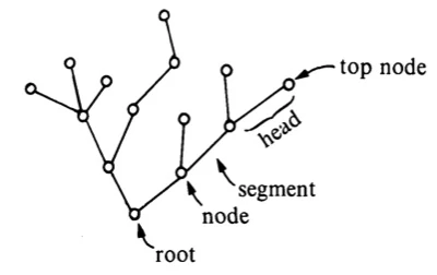
In the figure (Kirby and Paris, 1982), the leftmost top node is \(m(3)\), because it is the 3rd node up from the root. The node one segment below it is \(m(2)\), and it has 3 \(m(3)\) above, and therefore it is \(m(3)^3 m(2)\). The node below it is \(m(1)\) node with \(m(3)^3 m(2)\) and \(m(4)m(3)m(2)\), and therefore \([m(3)^3 m(2)][m(4)m(3)m(2)]m(1)\). The root node is \([m(2)[m(3)^2 m(2)]m(1)]\;[[m(3)^3 m(2)][m(4)m(3)m(2)]m(1)]\;(x)\).

In this figure, after cutting one of the top nodes at the \(m(3)\) level, 2 new hydra trees were produced from a node. It corresponds to evaluating \(m(3)=m(2)^x\) with \(x=3\). By comparing the \(m(n)\) structure to the hydra tree before and after cutting the heads,

\[[m(3)^2m(2)m(1)]^2[[m(3)^3m(2)][m(4)m(3)m(2)]m(1)](3) \\ = [[m(3)m(2)]^3m(1)][m(3)^2m(2)m(1)][[m(3)^3m(2)][m(4)m(3)m(2)]m(1)](3)\]

it exactly matches the definition of \(m(n)\) map, because

\[m(3)^2m(2)m(1)(3) = m(2)^3[m(3)m(2)]m(1)(3) \\ = [m(3)m(2)]^3m(1)(3)\]

\(m(n)\) map can thus be correlated with the hydra tree, which is correlated with ordinal of Cantor normal form (see the cited paper of Kirby and Paris, 1982). Therefore, it has the growth rate of \(f_{\varepsilon_0}(x)\).

See also

Googology in Asia

Indian counting system: Lakh · Crore · Tallakshana · Uppala · Dvajagravati · Paduma · Mahakathana · Asankhyeya · Dvajagranisamani · Vahanaprajnapti · Inga · Kuruta · Sarvanikshepa · Agrasara · Uttaraparamanurajahpravesa · Avatamsaka Sutra · Nirabhilapya nirabhilapya parivarta · Jaghanya Parīta Asaṃkhyāta
Chinese, Japanese and Korean counting system: Wan · Yi · Zhao · Jing · Gai · Zi · Rang · Gou · Jian · Zheng · Zai · Ji · Gougasha · Asougi · Nayuta · Fukashigi · Muryoutaisuu
See also: Template:Googology in Japan